A New Path for Artificial Intelligence
Dive into AXIOM, a revolutionary AI that learns like a human—efficiently, intuitively, and transparently. It challenges the foundations of modern deep learning by mastering complex games in minutes, not millennia, without relying on neural networks, backpropagation, or gradient-based optimization.
The AI Efficiency Crisis
Modern AI, particularly Deep Reinforcement Learning (DRL), is powerful but incredibly data-hungry. While a human can learn a new game in minutes, a DRL agent often needs billions of interaction steps—"tens of thousands of years of game play"[2]. This section frames the problem AXIOM was built to solve, contrasting the two dominant philosophies in the quest for more efficient AI.
The "Scale" Philosophy
This approach tackles inefficiency by building bigger, faster neural networks and training them with immense computational power and data. It pushes the current paradigm to its absolute limits, seeking intelligence through sheer capacity.
Method: Brute-force computation, massive function approximators.
Example: BBF (Bigger, Better, Faster)[11]
The "Structure" Philosophy
This approach argues that the key to intelligence lies in building AI with more explicit, human-like cognitive structures. Models learn an internal "world model," enabling them to "imagine," reason, and plan with far greater data efficiency.
The Anatomy of AXIOM
AXIOM is not a monolithic black box. It's a "modular 'digital brain'"[13] composed of four distinct yet interconnected mixture models. They work in concert to transform raw pixels into structured knowledge and goal-directed action, mirroring a logical decomposition of cognitive functions: perception, recognition, prediction, and reasoning. Click any module to learn more.
1. Slot Mixture Model (SMM)
Perception: Deconstructs a raw image into a set of distinct "objects" or slots, separating entities from the background.
2. Identity Mixture Model (iMM)
Recognition: Takes the discovered objects and classifies them into types (e.g., "ball", "paddle") based on their features like color and shape.
3. Transition Mixture Model (tMM)
Prediction: Acts as a "physics engine," modeling how objects can move with a library of simple motion primitives (e.g., "fall", "bounce").
4. Recurrent Mixture Model (rMM)
Reasoning: The cognitive core. It infers *why* an object moves in a certain way by modeling the causal rules of interaction and context.
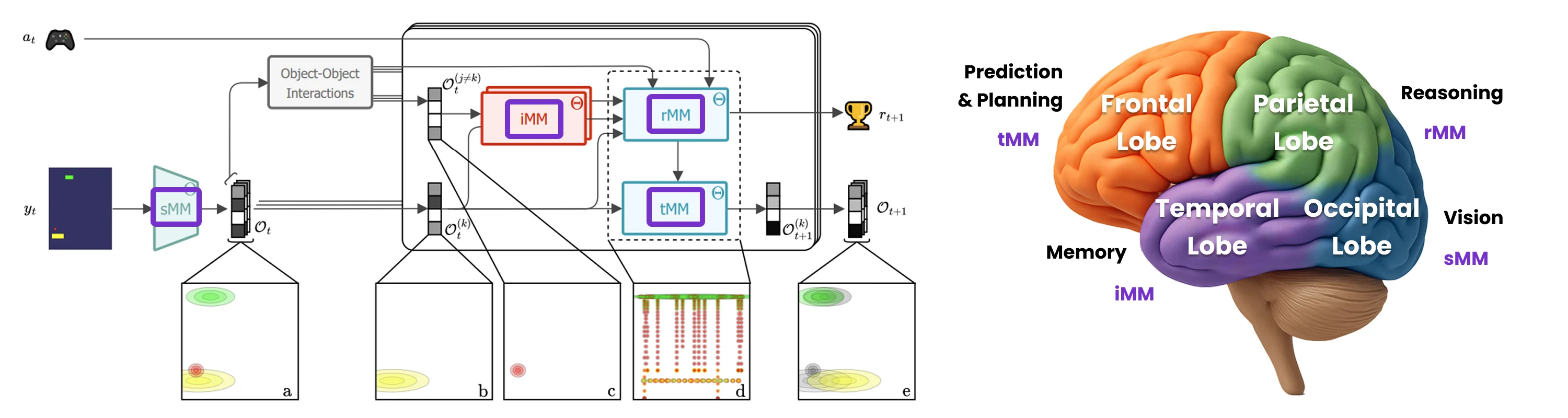
Figure 1: Inference and prediction flow using AXIOM: The sMM extracts object-centric representations from pixel inputs. For each object latent and its closest interacting counterpart, a discrete identity token is inferred using the iMM and passed to the rMM, along with the distance and the action, to predict the next reward and the tMM switch. The object latents are then updated using the tMM and the predicted switch to generate the next state for all objects. (a) Projection of the object latents into image space. (b) Projection of the kth latent whose dynamics are being predicted and (c) of its interaction partner. (d) Projection of the rMM in image space; each of the visualized clusters corresponds to a particular linear dynamical system from the tMM. (e) Projection of the predicted latents. The past latents at time t are shown in gray.
Source: AXIOM Digital Brain Whitepaper
SMM: From Pixels to Objects
The SMM is AXIOM's perceptual front-end. It takes a raw image, treats it as a collection of pixel tokens (each with RGB color and X,Y coordinates), and uses a Gaussian Mixture Model (GMM) to probabilistically group these pixels into a set of 'slots'. Each slot is an object-centric representation. Crucially, unlike methods like Slot Attention[14] that use iterative attention over CNN feature maps, the SMM is a more direct, probabilistic model where a slot's latent state (position, color, shape) *directly* defines the parameters of its corresponding Gaussian component. This creates a tight, interpretable link between the abstract representation and its visual manifestation.[1]
The Mathematics Behind Object Discovery
Step 1: From Pixels to Tokens
The SMM starts by converting each image into a collection of enriched pixel tokens. For an image of size H × W pixels:
Each token y_t^n contains both the visual information (RGB values) and spatial context (normalized X,Y coordinates) of pixel n at time t.
Step 2: The Mixture Model Architecture
The core insight is that pixels belonging to the same object should cluster together. The SMM models this using a Gaussian Mixture Model where each "slot" k corresponds to one object:
Each z_{t,k,smm}^n ∈ {0,1} is a binary indicator: "Does pixel n belong to slot k?"
Each x^{(k)} is a continuous vector encoding the object's position, color, and shape properties.
Step 3: Gaussian Components
Each slot defines a Gaussian distribution over pixel features. The beauty lies in how the slot's latent state directly parameterizes this Gaussian:
The mean directly extracts position and color from the slot latent.
The covariance encodes the object's spatial extent (shape) and color variance.
Step 4: Learning Through Variational Inference
The SMM learns by alternating between two steps:
For each pixel, calculate the probability it belongs to each slot and make soft assignments.
Given pixel assignments, update each slot's parameters to best explain its assigned pixels.
The Key Insight
Unlike attention-based methods that iteratively compete for pixels, the SMM creates a direct, interpretable mapping between abstract object properties (position, color, shape) and their visual manifestation. Each slot's latent state literally defines the parameters of a Gaussian "blob" in pixel space, making the model's internal representations inherently meaningful and manipulable.
@dataclass(frozen=True)
class SMMConfig:
    """Configuration for the Slot Mixture Model"""
    width: int = 160
    height: int = 210
    input_dim: int = 5  # RGB + X,Y coordinates
    slot_dim: int = 2   # Latent dimension per slot
    num_slots: int = 32 # Number of object slots
    use_bias: bool = True
    # ... other config parameters ...

def add_position_encoding(img):
    """Add X,Y coordinates to each pixel"""
    u, v = jnp.meshgrid(jnp.arange(img.shape[1]), jnp.arange(img.shape[0]))
    data = jnp.concatenate([
        (u.reshape(-1, 1)),
        (v.reshape(-1, 1)),
        img.reshape(-1, img.shape[-1]),
    ], axis=1)
    return data

def infer_and_update(key, smm, inputs, qx_prev, num_slots, **kwargs):
    """Core inference and update loop"""
    # Format input with position encoding
    inputs = _inputs_to_delta(inputs[None, ...])

    # E-step: Update slot assignments
    e_step_scan_fn = create_e_step_fn(smm, inputs)
    (qx, qz, ell_max), _ = lax.scan(e_step_scan_fn, init, jnp.arange(num_e_steps))

    # Get hard assignments and track used slots
    assignments = qz.argmax(-1)
    counts = jnp.bincount(assignments.ravel(), minlength=num_slots)
    used_component_idx = counts != 0

    # Grow model if needed
    smm_updated, qx_updated, qz_updated, ell_max_updated, used_updated, tries, done = grow_loop(
        smm, qx, qz, ell_max, used_component_idx, max_grow_steps
    )

    # Return updated model and variational parameters
    py = smm_updated.model.likelihood.variational_forward(qx_updated)
    return smm_updated, py, qx_updated, qz_updated, used_updated, ell_max_updated
Key Implementation Details:
- The model takes raw images and adds X,Y coordinates to each pixel, creating a 5D input (RGB + position)
- Each slot is represented by a Gaussian component in the mixture model
- The inference loop alternates between E-steps (updating slot assignments) and M-steps (updating slot parameters)
- The model can grow dynamically by adding new slots when needed, controlled by
the
eloglike_threshold - All operations are implemented in JAX for efficient GPU acceleration
iMM: What Am I Seeing?
Once objects are segmented by the SMM, the iMM answers, "What kind of objects are these?" It takes the continuous features of the slots (specifically, their 5-dimensional color and shape vectors) and assigns a discrete identity code to each one using another GMM. For example, it might learn that all small, red, circular objects belong to "type 1" (cherries) and all long, yellow, rectangular objects are "type 2" (paddles). This is vital for generalization, as it allows AXIOM to learn physical laws for an object *type*, not just for one specific instance, so it doesn't have to re-learn that all cherries fall down every time it sees a new one.[1]
From Continuous Features to Discrete Identities
Step 1: The Identity Challenge
The iMM solves a crucial abstraction problem: how to map continuous object features to discrete object types for type-specific rather than instance-specific learning.
5D feature vector: color (c) + shape (e) features per slot k
Step 2: The Generative Model
The iMM models these 5D features as a mixture of up to V Gaussian components, where each component represents a distinct object type:
Each z_{i,type}^{(k)} indicates which of the V object types is assigned to slot k.
Each type j has parameters μ_{j,type}, Σ_{j,type} for its feature distribution.
Step 3: Bayesian Priors
The model uses conjugate Normal-Inverse-Wishart (NIW) priors for robust parameter estimation:
This prior provides principled uncertainty quantification and prevents overfitting with limited data.
Step 4: Adaptive Type Discovery
The iMM can dynamically discover new object types using a stick-breaking process:
The parameter α₀,type controls the propensity to create new object types when encountering novel features.
Step 5: Type-Specific Learning
Without the iMM, each object slot would learn its own physics independently, requiring massive data.
Ball₂ → Physics₂
Ball₃ → Physics₃
With the iMM, all objects of the same type share dynamics, enabling rapid generalization.
The Key Innovation
The iMM enables compositional generalization by creating a shared type system. Once AXIOM learns that "red round objects bounce," this knowledge applies to all red round objects, not just the specific instances it trained on. This dramatically reduces the data requirements and enables rapid adaptation to new scenarios.
@dataclass(frozen=True)
class IMMConfig:
    """Configuration for the Identity Mixture Model"""
    num_object_types: int = 32
    num_features: int = 5
    i_ell_threshold: float = -500
    cont_scale_identity: float = 0.5
    color_precision_scale: float = 1.0
    color_only_identity: bool = False

def infer_identity(imm, x, color_only_identity=False):
    """Infer object identity from features"""
    # Extract and weight color features more heavily
    x = x[:, -5:, :]  # (x: (B, 11, 1) -> (B, 5, 1))
    object_features = x[:, :].at[:, 2:].set(x[:, 2:] * 100)
    object_features = object_features[:, 2 * int(color_only_identity):]

    # Compute log-likelihood and mask unused components
    _, c_ell, _ = imm.model._e_step(object_features, [])
    i_used_mask = imm.model.prior.alpha > imm.model.prior.prior_alpha
    elogp = (c_ell) * i_used_mask + (1 - i_used_mask) * (-1e10)

    # Get class assignments
    qz = softmax(elogp, imm.model.mix_dims)
    class_labels = qz.argmax(-1)
    return class_labels

def infer_remapped_color_identity(imm, obs, object_idx, num_features, **kwargs):
    """Infer identity based on shape when color-based inference fails"""
    object_features = obs[object_idx, None, obs.shape[-1] - num_features:, None]
    object_features = object_features.at[:, 2:, :].set(
        object_features[:, 2:, :] * 100
    )

    # Try color-based inference first
    _, c_ell, _ = imm.model._e_step(object_features, [])
    i_used_mask = imm.model.prior.alpha > imm.model.prior.prior_alpha
    ell = (c_ell) * i_used_mask + (1 - i_used_mask) * (-1e10)

    def _infer_based_on_features():
        return jax.nn.softmax(ell)[0]

    def _infer_based_on_shape():
        # Calculate likelihood using shape features only
        data = object_features[:, :2, :]
        mean = imm.model.continuous_likelihood.mean[:, :2, :]
        expected_inv_sigma = imm.model.continuous_likelihood.expected_inv_sigma()[:, :2, :2]
        # ... compute shape-based likelihood ...
        qz = jax.nn.softmax(100 * ell)
        return qz

    # Choose inference method based on confidence
    qz = jax.lax.cond(
        ell.max() > -100,
        _infer_based_on_features,
        _infer_based_on_shape
    )
    return qz
Key Implementation Details:
- The model uses a Hybrid Mixture Model to classify objects based on their features
- Color features are weighted 100x more heavily than shape features for better separation
- Includes a fallback mechanism to infer identity based on shape when color-based inference fails
- Maintains a mask of "used" object types to track which identities are active
- Supports both color-only and full feature-based identity inference
tMM: The "Physics Engine"
The tMM provides AXIOM with a predictive "physics engine." It is formulated as a switching linear dynamical system (SLDS). Instead of learning one highly complex function for all motion, the tMM maintains a shared library of up to L simple, linear motion primitives (e.g., "falling under gravity," "moving left," "bouncing"). For each object, a discrete switch variable selects a primitive from this library to predict its state at the next timestep. By switching between these simple modes, the tMM can approximate highly complex, non-linear trajectories. This shared library creates a compact, general-purpose physics engine applicable to any object based on context.[1]
Switching Linear Dynamical Systems for Physics
Step 1: The Switch Variable
The tMM's core innovation is the discrete switch variable that selects which linear dynamics to apply to each slot at each timestep:
Switch variable for slot k selects from L linear motion primitives
Step 2: The Generative Model
Each motion primitive is a linear transformation that predicts the next state. The full generative model is:
Each D_l is a matrix that defines a specific motion pattern (e.g., constant velocity, gravity).
Each b_l allows for non-zero baseline motion (e.g., constant acceleration).
Step 3: Shared Motion Library
The key insight is that all slots share the same library of motion primitives, enabling generalization across objects:
All components share the same noise level
All dynamics start with equal probability
Step 4: Adaptive Growth with Stick-Breaking
The tMM can dynamically discover new motion primitives using a stick-breaking prior:
The parameter α₀,tmm controls how readily new motion primitives are created when existing ones fail to explain observed transitions.
Step 5: Cross-Slot Learning
The revolutionary aspect is that motion primitives are shared across all slots, not slot-dependent:
Each object learns its own dynamics independently, requiring massive amounts of data.
Slot₂ → {D₂₁, D₂₂, ...}
Slot₃ → {D₃₁, D₃₂, ...}
All slots share the same library of motion primitives, enabling rapid learning of universal physics.
"Gravity", "Bounce", "Drift"
Step 6: Context-Dependent Switching
The switch variable is not random—it's predicted by the rMM based on context:
The rMM predicts which motion primitive to use based on object interactions, actions, and context
The Key Innovation
The tMM's genius lies in decomposing complex non-linear dynamics into a library of simple linear components. Instead of learning one massive function that handles all possible motions, it learns many simple functions and intelligently switches between them. This creates a modular, interpretable physics engine where each component has a clear meaning (e.g., "falling", "bouncing", "drifting") and can be shared across all objects in the scene.
@dataclass(frozen=True)
class TMMConfig:
    """Configuration for the Transition Mixture Model"""
    n_total_components: int = 200  # Maximum number of motion primitives
    state_dim: int = 2            # Dimension of state space (e.g., 2 for X/Y)
    dt: float = 1.0              # Time step
    sigma_sqr: float = 2.0       # Variance of Gaussian likelihood
    logp_threshold: float = -0.00001  # Threshold for adding new components
    position_threshold: float = 0.15  # Threshold for detecting teleportation
    use_velocity: bool = True    # Whether to use velocity-based dynamics

def generate_default_dynamics_component(state_dim, dt=1.0, use_bias=True):
    """Generate a constant velocity motion primitive"""
    # Encode constant velocity assumption
    velocity_coupling = jnp.eye(state_dim)
    base_transitions = block_diag(jnp.eye(state_dim), velocity_coupling)
    transition_matrix = jnp.pad(base_transitions, [(0, 0), (0, 1)])
    transition_matrix = transition_matrix.at[:state_dim, state_dim:-1].set(
        jnp.diag(dt * jnp.ones(state_dim))
    )
    return transition_matrix

def create_velocity_component(x_current, x_next, dt=1.0, use_unused_counter=True):
    """Create a new velocity-based motion primitive"""
    state_dim = x_current.shape[-1] // 2
    base_dynamics = generate_default_dynamics_component(
        state_dim=state_dim, dt=dt, use_bias=True
    )
    # Calculate velocity and bias
    vel = x_next[:state_dim] - x_current[:state_dim]
    prev_vel = x_current[state_dim:]
    vel_bias = vel - prev_vel

    # Create new component with calculated velocity
    new_component = base_dynamics.at[:, -1].set(
        jnp.concatenate(2 * [vel_bias])
    )
    return new_component

def update_transitions(transitions, x_prev, x_curr, used_mask, sigma_sqr=2.0,
                      logp_thr=-0.001, pos_thr=0.5, dt=1.0, use_velocity=True):
    """Update the transition model with new observations"""
    # Compute log probabilities for all components
    logprobs_all = compute_logprobs(
        transitions, x_prev, x_curr, sigma_sqr, use_velocity
    )

    # Mask unused components
    logprobs_used = jnp.where(used_mask, logprobs_all, -jnp.inf)
    max_used = logprobs_used.max()

    # Add new component if needed
    def add_component_case(trans):
        return add_vel_or_bias_component(
            trans, x_prev, x_curr, used_mask, pos_thr,
            dt=dt, use_velocity=use_velocity
        )

    transitions = jax.lax.cond(
        max_used < logp_thr,
        add_component_case,
        lambda x: x,
        transitions
    )

    # Update used mask and recompute probabilities
    used_mask = jnp.sum(jnp.abs(transitions), axis=(-1, -2)) > 0
    return transitions, used_mask, logprobs_used
Key Implementation Details:
- Uses a Switching Linear Dynamical System (SLDS) to model object motion
- Maintains a library of up to 200 motion primitives (constant velocity, teleportation, etc.)
- Each primitive is a linear transformation matrix that predicts the next state
- Automatically adds new motion primitives when existing ones can't explain the observed motion
- Supports both velocity-based and position-based dynamics
- Includes special handling for teleportation events (sudden position changes)
rMM: The Causal Reasoner
The rMM is the cognitive core where high-level reasoning occurs. Its main job is to infer the correct switch state for the tMM—that is, to answer: "Given the situation, which motion primitive should apply to this object now?" To do this, it acts as a sophisticated causal reasoning engine, implemented as a generative mixture model. It considers a rich context for a "focal" object: its own state (position, velocity), interaction features (distance to nearest neighbor and that neighbor's identity), the action taken by the agent, and the reward received. By learning a joint probability distribution over these variables, it discovers rules like, "If the paddle (type 2) is very close to the ball (type 1), and the agent moves up, then the tMM switch for the ball should be 'bouncing up'."[1]
Causal Reasoning Through Mixed Continuous-Discrete Modeling
Step 1: The Assignment Variable
The rMM uses a per-slot latent assignment variable to select which "causal rule" (mixture component) explains the current context:
Binary assignment vector for slot k, component m
Step 2: Mixed Feature Representation
The rMM models both continuous and discrete features to capture the full context (Equation 6):
Own state + interaction features
Identities, actions, rewards, switches
Step 3: The Generative Model
The rMM models the joint distribution over continuous and discrete features using a mixture of Gaussian and Categorical distributions (Equation 7):
Models continuous features like position, velocity, and distances with parameters μ_{m,rmm}, Σ_{m,rmm}.
Models discrete features like object identities, actions, and rewards with parameters α_{m,i}.
Step 4: Interaction Feature Engineering
The rMM uses sophisticated feature engineering to capture object interactions:
Selects relevant slot features
Computes slot-to-slot interactions
Step 5: Causal Rule Discovery
Each mixture component represents a distinct "causal rule" that explains when certain dynamics occur:
IF paddle close to ball AND action = "up" THEN ball dynamics = "bounce up"
• Distance < threshold
• Identity = paddle + ball
• Action = up
• Switch = bounce_up
IF no interactions AND no action THEN object dynamics = "gravity"
• Distance > threshold
• Action = none
• Switch = gravity
Step 6: Adaptive Growth
Like other AXIOM components, the rMM can discover new causal rules using stick-breaking:
New causal rules are added when existing components cannot explain novel context-action-outcome patterns.
Step 7: Prediction and Planning
The rMM enables both prediction and planning by modeling the joint distribution:
Given context and action, predict tMM switch and expected reward.
Given context and desired outcome, infer which action to take.
The Key Innovation
The rMM's breakthrough is learning causal rules that connect context, actions, and outcomes in a generative framework. Unlike discriminative models that only map inputs to outputs, the rMM models the full joint distribution, enabling both prediction ("what will happen if I do X?") and planning ("what should I do to achieve Y?"). This bidirectional reasoning, combined with the ability to discover new causal rules online, makes AXIOM a truly causal reasoning system.
def _to_distance_obs_hybrid(
    imm, data, object_idx, action, reward, tmm_switch,
    tracked_obj_mask, interact_with_static, ...
):
    # Determine interacting object by checking for ellipse overlap
    other_idx, distances = get_interacting_objects_ellipse(
        data, tracked_obj_mask, object_idx, ...
    )

    # Infer identity of self and other object using the iMM
    self_id = nn.one_hot(object_identities[object_idx], ...)
    other_id = nn.one_hot(
        jax.lax.cond(other_idx == -1, lambda: num_object_classes, ...), ...
    )

    # Continuous features: (x, y, u, vx, vy, dist_x, dist_y)
    c_feat = data[object_idx, :5]
    d = distances[other_idx]
    c_feat = jnp.concatenate([c_feat, d], axis=0)

    # Discrete features: self_id, other_id, action, reward, tmm_switch
    d_feat = [
        self_id, other_id, nn.one_hot(action, ...),
        nn.one_hot((reward + 1).astype(jnp.int32), ...),
        nn.one_hot(tmm_switch, ...),
    ]
    return c_feat, d_feat

def predict(
    rmm: RMM, c_sample: Array, d_sample: List[Array], key: Array = None, ...
):
    # Overwrite switch and reward observations with a uniform prior
    d_sample = d_sample[:-2] + [jnp.ones_like(d[-i]) * 1/d[-i].size for i in [2, 1]]

    # Do an E-step to infer the mixture cluster (the causal rule)
    qz, c_ell, d_ell = rmm.model._e_step(c_sample, d_sample)
    elogp = c_ell + d_ell
    elogp = elogp * rmm.used_mask[None] + (1 - rmm.used_mask[None]) * (-1e10)
    qz = softmax(elogp, rmm.model.mix_dims)

    # Sample or pick the most likely mixture component
    mix_slot = jr.choice(key, qz[0].shape[0], p=qz[0]) if key else qz[0].argmax(-1)

    # Get the distribution over the TMM switch for the inferred cluster
    p_tmm = rmm.model.discrete_likelihoods[-1].mean()[..., 0]
    tmm_slot = p_tmm[mix_slot].argmax(-1)

    # Predict the reward, being optimistic about positive rewards
    p_reward = rmm.model.discrete_likelihoods[-2].mean()[..., 0]
    max_likelihood_reward = p_reward[mix_slot]
    reward = jax.lax.cond(
        max_likelihood_reward[-1] > reward_prob_threshold,
        lambda: 1.0,
        lambda: jnp.dot(jnp.array([-1.0, 0.0, 1.0]), jnp.dot(qz[0], p_reward)),
    )
    return tmm_slot[None], reward[None], ...
Key Implementation Details:
- The function
_to_distance_obs_hybridassembles the rich contextual input vector for reasoning. This includes the object's own state, interaction features (e.g., relative distance to a neighbor), its identity, the other object's identity, the action taken, and the resulting reward. - Interactions are determined by calculating ellipse overlaps
(
get_interacting_objects_ellipse), providing a simple but effective physical heuristic. - The
predictfunction performs an E-step on the mixture model to find the most likely "causal rule" (mixture component) that explains the current context. - Based on this inferred rule, it predicts the most probable motion primitive
(
tmm_slot) and the expected reward. - Reward prediction uses an optimistic heuristic: if the most likely outcome has a high probability of positive reward, predict 1.0; otherwise, calculate the expectation. This biases the agent towards potentially rewarding actions.
Learning and Deciding
AXIOM's learning process is as unique as its architecture. It learns online, one frame at a time, in a dynamic dance of growth and simplification. Its decisions are guided by a single, powerful principle: Active Inference.
Adaptive Growth & Pruning
AXIOM starts with a minimal model. When it encounters something novel or surprising (a new object, a new type of movement), it grows its internal models by adding a new component—a new "hypothesis" to explain the phenomenon. This is Adaptive Growth. To prevent just memorizing everything, it periodically engages in Bayesian Model Reduction (BMR), a pruning process that merges redundant or overly specific hypotheses into a single, more general rule. This explicit cycle of hypothesis generation and theory simplification is how AXIOM generalizes from limited data.[1]
Planning with Active Inference
AXIOM plans by selecting policies (sequences of actions) that are expected to minimize Expected Free Energy (G). This elegantly unifies two drives: seeking rewards and seeking information.[1]
Pragmatic Value (Exploitation): The first term drives the agent to seek states it expects to be rewarding (maximizing utility).
Epistemic Value (Exploration): The second term (a KL Divergence) is a formalization of curiosity. It drives the agent to take actions that are expected to resolve its uncertainty about how the world works (maximizing information gain).
Putting AXIOM to the Test
The Gameworld 10k benchmark was designed to test the limits of fast learning. With a strict budget of just 10,000 interactions (a few minutes of gameplay), agents must learn complex object-based dynamics from pixels. The charts below compare AXIOM to two state-of-the-art deep learning models: the structured, model-based DreamerV3 and the scaled-up, model-free BBF.
Gameworld 10k: Cumulative Reward
This chart shows the final score achieved by each model across 10 games after 10,000 steps. Higher scores are better. AXIOM consistently attains higher, or on-par, average cumulative reward in every environment.[1, Table 1]
Model Size: Parameters
This chart compares the number of learnable parameters for each model (on a logarithmic scale). AXIOM's model is orders of magnitude smaller—up to 440 times smaller than DreamerV3 and 7 times smaller than BBF—making it lighter and more efficient.[1, Table 2]
Computational Speed
This chart shows how long it takes each model to perform its core update step. AXIOM's gradient-free variational Bayesian update is substantially faster than the backpropagation used by deep learning models.[1, Table 2]
The "Glass Box" Advantage
Beyond performance, AXIOM's greatest strength is its transparency. Unlike opaque "black box" neural networks, AXIOM's internal states are interpretable, allowing for unprecedented analysis and even direct, surgical intervention.
Case Study: Cognitive Surgery
In a perturbation experiment, researchers suddenly changed the colors of game objects mid-training. A traditional AI would suffer catastrophic failure, its entangled representation of appearance and dynamics rendered useless. With AXIOM, the developers could pinpoint the problem and perform a "cognitive intervention."[1, Appx. E.3]
Diagnosis: The developers could see the failure point was precisely localized to the Identity Model (iMM), which uses color to infer object identity. The new, unseen colors were causing it to create new object types with no associated physics.
Intervention: Instead of costly retraining, they performed a "cognitive surgery" by surgically modifying the iMM's inference process, instructing it to temporarily ignore color information and rely solely on shape to determine object identity.
Result: The model instantly re-associated the color-changed objects with their original identities. The entire library of previously learned dynamics and causal rules in the tMM and rMM became immediately applicable again. Performance was rescued with no retraining required.
This functional interpretability, which allows a human to act as a "cognitive debugger," is simply not possible with today's black-box systems and highlights a path toward building safer, more reliable AI.
A Glimpse of the Future
AXIOM is more than a new model; it's a compelling argument that the path to more general and efficient AI may lie in structure, not just scale. By combining principled Bayesian inference with strong, object-centric priors, it achieves remarkable performance while remaining lightweight, transparent, and adaptable. While it currently relies on engineered priors, the quest to have AI learn these structures autonomously marks the next exciting frontier. AXIOM offers a glimpse of what that future might look like: structured, curious, efficient, and, above all, understandable.
References
A comprehensive list of papers and resources referenced in this report.
Core Papers
World Models & Object-Centric Learning
Object-Centric Representations
Test Your Understanding
Challenge yourself with this interactive quiz about AXIOM's architecture, principles, and capabilities. Each question is designed to deepen your understanding of the key concepts.
Question 1
Hint:
Quiz Complete!
You've completed all questions about AXIOM.
Critical Thinking: Deeper Questions
Beyond the impressive results, AXIOM's approach raises profound questions about the nature of intelligence, scalability, and the path toward artificial general intelligence. Explore these thought-provoking questions that challenge the boundaries of what we've learned.
The Question
AXIOM's four-module system (SMM, iMM, tMM, rMM) is a functional decomposition of cognition. However, the brain's architecture is also highly anatomical, featuring specialized structures for different types of memory (e.g., the hippocampus for episodic memory), emotional valuation (amygdala), and complex motor control (cerebellum). How might the absence of these distinct anatomical systems for memory and motivation limit AXIOM's ability to learn tasks that require not just understanding physics, but also recalling long-term narrative sequences or making decisions based on nuanced, emotionally-salient outcomes?
Consider:
- • How does AXIOM handle episodic memory?
- • Can it learn from emotional context?
- • What about complex motor sequences?
Implications:
- • Limitations in narrative understanding
- • Challenges with emotional reasoning
- • Gaps in long-term memory systems
The Bottleneck
The report states that AXIOM's greatest strength—its hand-engineered, object-centric priors—is also its greatest limitation. For AXIOM to replace a general-purpose deep learning model (like a Transformer, which can process diverse data types), a breakthrough is needed to "learn the priors." Does this imply that for any given domain (e.g., fluid dynamics, social interactions, abstract mathematics), a fundamentally different set of core priors is required? If so, does the AXIOM approach lead not to a single AGI, but to a "zoo" of highly specialized, non-interoperable intelligent systems?
Domain Examples
- • Fluid dynamics
- • Social interactions
- • Abstract mathematics
- • Language processing
Key Questions
- • One AGI or many specialists?
- • Can priors be learned?
- • Transfer between domains?
- • Interoperability challenges?
Implications
- • Scaling limitations
- • Engineering overhead
- • Generalization barriers
- • Alternative architectures?
The Scaling Challenge
AXIOM excels in Gameworld, where the number of objects and interaction rules is limited. Consider a real-world task like navigating a busy warehouse. The number of objects is vast, their states are complex (e.g., a deformable cardboard box), and the potential causal interactions are nearly infinite. How would AXIOM's learning mechanism, particularly the cycle of growing the model with new hypotheses (clusters) and then pruning it with Bayesian Model Reduction (BMR), cope with this combinatorial explosion? Could the model become computationally intractable, or would it risk over-generalizing and pruning away critical, rare-but-important causal rules?
Complexity Factors
Object Complexity
- • Thousands of objects
- • Deformable materials
- • Occlusion and lighting
- • Multi-scale interactions
Interaction Complexity
- • Infinite causal chains
- • Rare but critical events
- • Context-dependent rules
- • Emergent behaviors
Potential Failure Modes
Computational Intractability
Model growth outpaces computational resources, leading to exponential complexity.
Over-Generalization
BMR prunes away rare but critical causal rules, leading to brittle behavior.
The Representation Challenge
AXIOM's interpretability comes from its discrete, "glass-box" representations (e.g., this is "object type 1," using "motion primitive 3"). In contrast, deep learning models build high-dimensional, continuous representations where concepts can be subtly blended. Could AXIOM's reliance on discrete categories be a source of brittleness, making it difficult to capture the ambiguous, abstract, or metaphorical reasoning that humans excel at? For example, how would it represent a concept like "a threatening posture" which is not a discrete object but a continuous configuration of one?
Discrete Representations
Advantages
- • Clear interpretability
- • Explicit categories
- • Surgical intervention
- • Logical reasoning
Limitations
- • Hard categorical boundaries
- • Limited ambiguity handling
- • Difficulty with gradients
- • Metaphorical reasoning
Continuous Representations
Advantages
- • Smooth concept blending
- • Gradient representations
- • Ambiguity modeling
- • Metaphorical reasoning
Limitations
- • Black-box nature
- • Difficult to interpret
- • Hard to debug
- • Unpredictable behavior
Challenge Examples
Abstract Concepts
"Threatening posture" - not a discrete object but a configuration
Metaphorical Reasoning
Understanding "time is money" or "mind as computer"
Ambiguous Situations
Objects that blend categories or context-dependent meanings
The Path Forward
These questions don't diminish AXIOM's remarkable achievements, but rather illuminate the profound challenges that remain in our quest for artificial general intelligence. They remind us that each breakthrough in AI opens new questions as fascinating as the answers it provides.